Overview
In this lab we use a simulator to localize a robot using Bayes filter. To implement the filter, the map is broken into a grid of discrete cells. Then a motion model which predicts the likelihood of transtions between state is built. Supplementing a motion model is a measurement model that updates the belief based on sensor readings. Each step of the filter is broken into a prediction step which uses the motion model and adds uncertainty to the robot's pose and then an update step which incorporates the sensor readings and decreases the uncertainty. In the end, you have a grid of probabilities denoting the probability of the robot to be in each cell.
Compute Control
A motion command , u, can be desconstructed into three separate stages: initial rotation, translation, and final rotation. Compute_control uses the robot's current and past pose to get the ideal motion command.
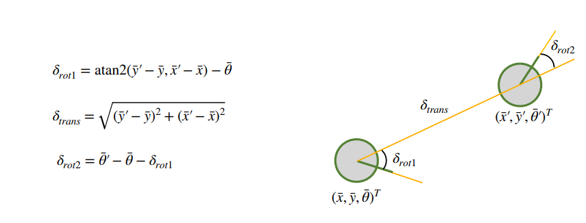
Compute Control
Artemis Code
Odometry Motion Model
The odometry motion model calculates the probability of transition from a previous state to a new state by comparing the ideal motion command (calculated by compute_control) to the actual odometry reading. The probability calculations are shown in the image below.
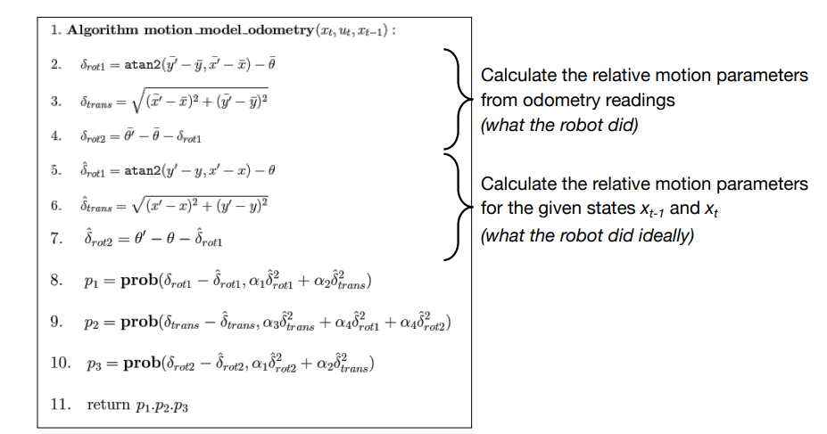
odom_motion_model
Artemis Code
Prediction Step
The prediction step uses the odometry to predict its new pose, implementing the equation: $$ \overline{bel}(x_t) = \sum_{x_{t-1}} p(x_t \mid x_{t-1}, u_t) \cdot bel(x_{t-1}) $$ We loop over every possible previous state (skipping states with probability below 0.0001 for computational efficiency) and calculate the probability of transitioning to each new state given the odometry reading. All probabilities are then normalized to sum to 1.
Prediction Step Code
Artemis Code
Sensor Model
The sensor model computes $p(z_t \mid x_t)$, the likelihood of the robot's 18 range measurements given a particular grid cell. For each of the 18 scan angles, a Gaussian is evaluated comparing the actual sensor reading $z_t^{(i)}$ against the expected reading $z_{true}^{(i)}$ pre-computed for that cell: $$ p(z_t \mid x_t) = \prod_{i=1}^{18} \mathcal{N}(z_t^{(i)};\, z_{true}^{(i)}(x_t),\, \sigma_{sensor}) $$ The function returns an array of 18 individual likelihoods, which are then multiplied together in the update step to get the total likelihood for that cell.
Sensor Model
Artemis Code
Update Step
In the update step, the measurements are incorporated to decrease uncertainty in the robot's pose: $$ bel(x_t) = \eta \cdot p(z_t \mid x_t) \cdot \overline{bel}(x_t) $$ where $p(z_t \mid x_t) = \prod_{i=1}^{18} \mathcal{N}(z_t^{(i)};\, z_{true}^{(i)}(x_t),\, \sigma_{sensor})$. We loop over every cell in the grid and compute the likelihood by comparing the 18 expected range measurements stored in the map against the robot's actual sensor readings. The belief is then normalized to sum to 1.
▸ update_step
Python Code
Simulation Results
Localization Video
Trajectory Plot
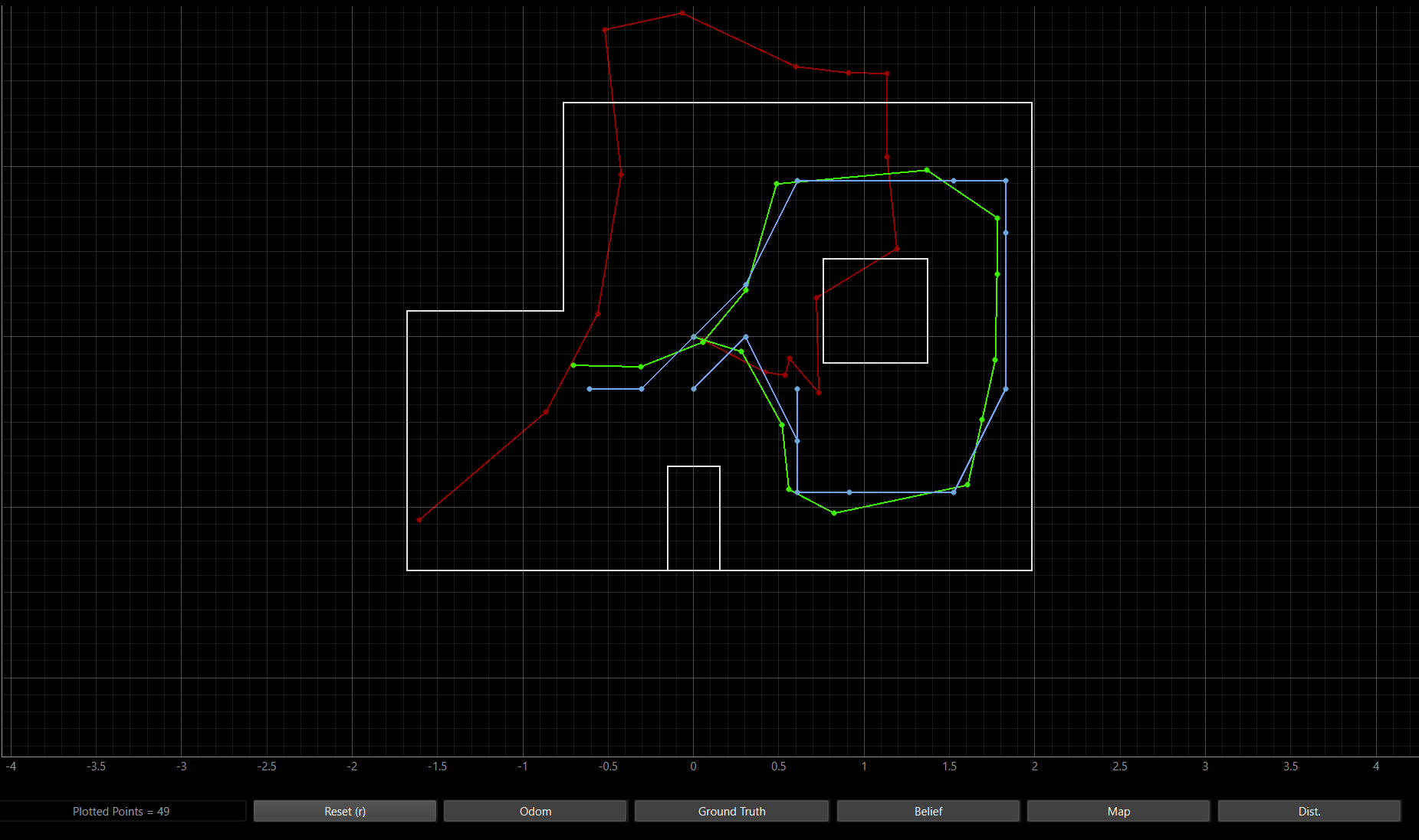
The trajectory plot shows that the predicted pose (shown in blue) closely tracked the ground truth (shown in green). The odometry readings (shown in red) were very noisy, at times showing the robot's pose as being outside of the world map. Nonethless, the the robot was effectively localized despite the noisy odometry readings.
Resources
I refrenced Stephen Wagner and Jack Long's code.